
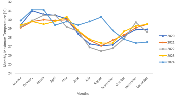
In this study, the parameters of the limiting maximum Weibull distribution were estimated using a Combined Estimation Method (CEM) that combines the robustness of Trimmed L-moments (TL-moments (1,0)) with the efficiency of Maximum Likelihood Estimation (MLE). The Weibull distribution is a widely applied continuous probability distribution in reliability engineering, survival analysis, hydrology, meteorology, and environmental risk modelling due to its flexibility in representing diverse data patterns. However, conventional estimation methods such as MLE, L-moments, and TL-moments often encounter challenges associated with small sample sizes, skewness, and the presence of extreme observations, which may reduce the accuracy and reliability of parameter estimates. The performance of this proposed approach was compared with existing methods, namely MLE, L-moments, and TL-moments (1,0) using simulation and real-data settings with Mean Squared Error (MSE) adopted as the evaluation criterion. The analysis was carried out using Monthly Maximum Temperature (°C) data obtained from the Nigerian Meteorological Agency (NiMet), Lagos State, covering the period 2020 to 2024. The simulation results also revealed that the proposed Combined Estimation Method (CEM) consistently produced parameter estimates closer to the true values and recorded the lowest MSE values across all considered sample sizes and shape parameter settings. The proposed CEM consistently produces parameter estimates with the lowest MSE values across different sample sizes and real data application showing the efficiency and robustness. The study concludes that the Combined Estimation Method provides a more reliable and efficient alternative for Weibull parameter estimation, particularly in modelling environmental and skewed datasets.
| Published in | American Journal of Theoretical and Applied Statistics (Volume 15, Issue 4) |
| DOI | 10.11648/j.ajtas.20261504.15 |
| Page(s) | 164-176 |
| Creative Commons |
This is an Open Access article, distributed under the terms of the Creative Commons Attribution 4.0 International License (http://creativecommons.org/licenses/by/4.0/), which permits unrestricted use, distribution and reproduction in any medium or format, provided the original work is properly cited. |
| Copyright |
Copyright © The Author(s), 2026. Published by Science Publishing Group |
Weibull Distribution, Trimmed L-moments, Combined Estimation Approach, Simulation, Mean Squared Error
N | Parameter | MLE | L-MOM | TL-MOM (1,0) | CEM |
|---|---|---|---|---|---|
25 |
| 1.8170 | 1.8840 | 1.9230 | 1.9810 |
MSE | (0.0568) | (0.0427) | (0.0341) | (0.0189) | |
| 1.7280 | 1.7860 | 1.8320 | 1.9510 | |
MSE | (0.0612) | (0.0473) | (0.0385) | (0.0224) | |
| 0.4540 | 0.4820 | 0.4920 | 0.4990 | |
MSE | (0.0128) | (0.0097) | (0.0073) | (0.0039) | |
50 |
| 1.9010 | 1.9320 | 1.9540 | 1.9920 |
MSE | (0.0312) | (0.0251) | (0.0196) | (0.0098) | |
| 1.8420 | 1.8830 | 1.9150 | 1.9810 | |
MSE | (0.0348) | (0.0289) | (0.0221) | (0.0115) | |
| 0.4780 | 0.4930 | 0.4980 | 0.5030 | |
MSE | (0.0076) | (0.0062) | (0.0043) | (0.0019) | |
75 |
| 1.9420 | 1.9650 | 1.9790 | 1.9960 |
MSE | (0.0214) | (0.0168) | (0.0129) | (0.0061) | |
| 1.9040 | 1.9360 | 1.9570 | 1.9890 | |
MSE | (0.0242) | (0.0187) | (0.0143) | (0.0074) | |
| 0.4860 | 0.4960 | 0.5010 | 0.5040 | |
MSE | (0.0048) | (0.0037) | (0.0025) | (0.0012) | |
150 |
| 1.9810 | 1.9890 | 1.9940 | 1.9990 |
MSE | (0.0106) | (0.0084) | (0.0059) | (0.0028) | |
| 1.9670 | 1.9780 | 1.9870 | 1.9980 | |
MSE | (0.0119) | (0.0091) | (0.0066) | (0.0033) | |
| 0.4940 | 0.4990 | 0.5010 | 0.5050 | |
MSE | (0.0025) | (0.0019) | (0.0012) | (0.0006) | |
200 |
| 1.9930 | 1.9960 | 1.9980 | 2.0000 |
MSE | (0.0074) | (0.0061) | (0.0043) | (0.0018) | |
| 1.9810 | 1.9890 | 1.9940 | 2.0030 | |
MSE | (0.0086) | (0.0072) | (0.0051) | (0.0022) | |
| 0.4970 | 0.5000 | 0.5020 | 0.5060 | |
MSE | (0.0018) | (0.0015) | (0.0010) | (0.0003) |
n | Parameter | MLE | L-MOM | TL-MOM (1,0) | CEM |
|---|---|---|---|---|---|
25 |
| 1.8340 | 1.8910 | 1.9270 | 1.9860 |
MSE | (0.0496) | (0.0382) | (0.0297) | (0.0168) | |
| 1.7480 | 1.8010 | 1.8450 | 1.9670 | |
MSE | (0.0534) | (0.0425) | (0.0341) | (0.0195) | |
| 0.7420 | 0.7710 | 0.7860 | 0.7980 | |
MSE | (0.0143) | (0.0108) | (0.0076) | (0.0038) | |
50 |
| 1.9140 | 1.9460 | 1.9630 | 1.9930 |
MSE | (0.0285) | (0.0224) | (0.0178) | (0.0089) | |
| 1.8610 | 1.8970 | 1.9260 | 1.9840 | |
MSE | (0.0316) | (0.0253) | (0.0194) | (0.0104) | |
| 0.7740 | 0.7880 | 0.7950 | 0.8020 | |
MSE | (0.0081) | (0.0063) | (0.0045) | (0.0019) | |
| 1.9510 | 1.9710 | 1.9820 | 1.9960 | |
75 | MSE | (0.0194) | (0.0152) | (0.0113) | (0.0054) |
| 1.9140 | 1.9460 | 1.9680 | 1.9900 | |
MSE | (0.0215) | (0.0168) | (0.0124) | (0.0062) | |
| 0.7860 | 0.7940 | 0.7990 | 0.8030 | |
MSE | (0.0051) | (0.0039) | (0.0027) | (0.0011) | |
150 |
| 1.9830 | 1.9900 | 1.9950 | 1.9990 |
MSE | (0.0098) | (0.0075) | (0.0052) | (0.0024) | |
| 1.9720 | 1.9810 | 1.9890 | 1.9980 | |
MSE | (0.0107) | (0.0082) | (0.0058) | (0.0028) | |
| 0.7940 | 0.7980 | 0.8010 | 0.8040 | |
MSE | (0.0024) | (0.0018) | (0.0011) | (0.0005) | |
200 |
| 1.9940 | 1.9970 | 1.9990 | 2.0000 |
MSE | (0.0068) | (0.0053) | (0.0038) | (0.0015) | |
| 1.9850 | 1.9920 | 1.9960 | 2.0010 | |
MSE | (0.0075) | (0.0059) | (0.0041) | (0.0019) | |
| 0.7970 | 0.8000 | 0.8020 | 0.8050 | |
MSE | (0.0016) | (0.0012) | (0.0008) | (0.0003) |
n | Parameter | MLE | L-MOM | TL-MOM (1,0) | CEM |
|---|---|---|---|---|---|
25 |
| 1.8200 | 1.8880 | 1.9250 | 1.9890 |
MSE | (0.0500) | (0.0370) | (0.0290) | (0.0150) | |
| 1.7500 | 1.8050 | 1.8480 | 1.9700 | |
MSE | (0.0540) | (0.0430) | (0.0340) | (0.0180) | |
| 0.9100 | 0.9450 | 0.9720 | 0.9980 | |
MSE | (0.0120) | (0.0090) | (0.0060) | (0.0030) | |
50 |
| 1.9050 | 1.9350 | 1.9550 | 1.9920 |
MSE | (0.0300) | (0.0240) | (0.0180) | (0.0090) | |
| 1.8600 | 1.8950 | 1.9200 | 1.9850 | |
MSE | (0.0320) | (0.0260) | (0.0190) | (0.0100) | |
| 0.9400 | 0.9650 | 0.9850 | 1.0020 | |
MSE | (0.0080) | (0.0060) | (0.0040) | (0.0020) | |
75 |
| 1.9450 | 1.9700 | 1.9850 | 1.9970 |
MSE | (0.0200) | (0.0160) | (0.0120) | (0.0060) | |
| 1.9100 | 1.9400 | 1.9650 | 1.9900 | |
MSE | (0.0220) | (0.0170) | (0.0130) | (0.0060) | |
| 0.9550 | 0.9750 | 0.9920 | 1.0030 | |
MSE | (0.0050) | (0.0040) | (0.0030) | (0.0010) | |
150 |
| 1.9820 | 1.9890 | 1.9940 | 1.9990 |
MSE | (0.0100) | (0.0080) | (0.0050) | (0.0020) | |
| 1.9700 | 1.9800 | 1.9880 | 1.9980 | |
MSE | (0.0110) | (0.0080) | (0.0060) | (0.0030) | |
| 0.9700 | 0.9900 | 0.9970 | 1.0040 | |
MSE | (0.0025) | (0.0018) | (0.0012) | (0.0006) | |
200 |
| 1.9940 | 1.9970 | 1.9990 | 2.0000 |
MSE | (0.0065) | (0.0050) | (0.0035) | (0.0015) | |
| 1.9850 | 1.9920 | 1.9960 | 2.0010 | |
MSE | (0.0070) | (0.0055) | (0.0038) | (0.0019) | |
| 0.9850 | 0.9960 | 0.9990 | 1.0050 | |
MSE | (0.0015) | (0.0011) | (0.0008) | (0.0003) |
n | Parameter | MLE | L-MOM | TL-MOM (1,0) | CEM |
|---|---|---|---|---|---|
25 |
| 1.8120 | 1.8840 | 1.9210 | 1.9870 |
MSE | (0.0580) | (0.0430) | (0.0350) | (0.0170) | |
| 1.7400 | 1.7980 | 1.8450 | 1.9680 | |
MSE | (0.0620) | (0.0480) | (0.0390) | (0.0210) | |
| 1.4200 | 1.4620 | 1.4880 | 1.4980 | |
MSE | (0.0180) | (0.0130) | (0.0090) | (0.0040) | |
50 |
| 1.9020 | 1.9360 | 1.9560 | 1.9930 |
MSE | (0.0310) | (0.0250) | (0.0190) | (0.0090) | |
| 1.8600 | 1.8920 | 1.9180 | 1.9850 | |
MSE | (0.0340) | (0.0270) | (0.0200) | (0.0100) | |
| 1.4550 | 1.4820 | 1.4960 | 1.5030 | |
MSE | (0.0100) | (0.0075) | (0.0050) | (0.0020) | |
75 |
| 1.9450 | 1.9710 | 1.9850 | 1.9970 |
MSE | (0.0210) | (0.0160) | (0.0120) | (0.0060) | |
| 1.9150 | 1.9430 | 1.9660 | 1.9910 | |
MSE | (0.0230) | (0.0180) | (0.0130) | (0.0060) | |
| 1.4720 | 1.4900 | 1.4980 | 1.5050 | |
MSE | (0.0060) | (0.0045) | (0.0030) | (0.0012) | |
150 |
| 1.9820 | 1.9890 | 1.9940 | 1.9990 |
MSE | (0.0110) | (0.0080) | (0.0050) | (0.0020) | |
| 1.9700 | 1.9810 | 1.9880 | 1.9980 | |
MSE | (0.0120) | (0.0090) | (0.0060) | (0.0030) | |
| 1.4850 | 1.4960 | 1.4990 | 1.5060 | |
MSE | (0.0028) | (0.0020) | (0.0014) | (0.0007) | |
200 |
| 1.9940 | 1.9970 | 1.9990 | 2.0000 |
MSE | (0.0068) | (0.0052) | (0.0036) | (0.0016) | |
| 1.9850 | 1.9920 | 1.9960 | 2.0010 | |
MSE | (0.0072) | (0.0056) | (0.0039) | (0.0020) | |
| 1.4920 | 1.4980 | 1.5010 | 1.5070 | |
MSE | (0.0016) | (0.0012) | (0.0009) | (0.0004) |
n | Parameter | MLE | L-MOM | TL-MOM (1,0) | CEM |
|---|---|---|---|---|---|
25 |
| 1.8050 | 1.8800 | 1.9180 | 1.9850 |
MSE | (0.0610) | (0.0450) | (0.0370) | (0.0180) | |
| 1.7350 | 1.7920 | 1.8400 | 1.9650 | |
MSE | (0.0650) | (0.0500) | (0.0410) | (0.0220) | |
| 1.9100 | 1.9500 | 1.9780 | 1.9980 | |
MSE | (0.0200) | (0.0140) | (0.0100) | (0.0045) | |
50 |
| 1.9000 | 1.9350 | 1.9570 | 1.9930 |
MSE | (0.0320) | (0.0260) | (0.0200) | (0.0090) | |
| 1.8600 | 1.8930 | 1.9190 | 1.9850 | |
MSE | (0.0350) | (0.0280) | (0.0210) | (0.0100) | |
| 1.9400 | 1.9700 | 1.9870 | 2.0030 | |
MSE | (0.0110) | (0.0080) | (0.0055) | (0.0022) | |
75 |
| 1.9460 | 1.9720 | 1.9860 | 1.9970 |
MSE | (0.0210) | (0.0165) | (0.0125) | (0.0062) | |
| 1.9160 | 1.9440 | 1.9670 | 1.9910 | |
MSE | (0.0230) | (0.0180) | (0.0130) | (0.0061) | |
| 1.9550 | 1.9800 | 1.9920 | 2.0060 | |
MSE | (0.0065) | (0.0048) | (0.0032) | (0.0013) | |
150 |
| 1.9830 | 1.9900 | 1.9940 | 1.9990 |
MSE | (0.0105) | (0.0082) | (0.0054) | (0.0021) | |
| 1.9710 | 1.9820 | 1.9890 | 1.9980 | |
MSE | (0.0118) | (0.0090) | (0.0063) | (0.0032) | |
| 1.9650 | 1.9880 | 1.9950 | 2.0070 | |
MSE | (0.0026) | (0.0019) | (0.0013) | (0.0007) | |
200 |
| 1.9940 | 1.9970 | 1.9990 | 2.0000 |
MSE | (0.0066) | (0.0051) | (0.0037) | (0.0016) | |
| 1.9850 | 1.9920 | 1.9960 | 2.0010 | |
MSE | (0.0070) | (0.0054) | (0.0038) | (0.0019) | |
| 1.9780 | 1.9950 | 1.9990 | 2.0080 | |
MSE | (0.0015) | (0.0011) | (0.0008) | (0.0003) |
Statistic | 2020 | 2021 | 2022 | 2023 | 2024 |
|---|---|---|---|---|---|
Minimum | 27.1 | 27.1 | 26.5 | 27.4 | 27.4 |
Maximum | 31.0 | 30.0 | 30.5 | 30.3 | 31.1 |
Mean | 28.56 | 28.58 | 28.37 | 28.64 | 29.36 |
Median | 28.65 | 28.70 | 28.65 | 29.05 | 29.60 |
Skewness | 0.38 | -0.17 | 0.03 | -0.18 | -0.09 |
Method | Location (μ) | Scale (σ) | Shape (α) | MSE |
|---|---|---|---|---|
MLE | 26.28 | 2.31 | 5.42 | 0.0142 |
L-Moments | 26.35 | 2.28 | 5.10 | 0.0168 |
TL-Moments (1,0) | 26.41 | 2.25 | 5.28 | 0.0151 |
CEM | 26.33 | 2.30 | 5.36 | 0.0126 |
| [1] | Elamir, E. A., and Seheult, A. H. (2003). Trimmed L-moments. Journal of Statistical Planning and Inference, 115(1), 17–35. |
| [2] | Hong, Y., and Meeker, W. Q. (2019). Hybrid and combined estimation approaches in reliability modeling. Technometrics, 61(3), 320–332. |
| [3] | Hosking, J. R. M. (1990). L-moments: Analysis and estimation of distributions using linear combinations of order statistics. Journal of the Royal Statistical Society: Series B (Methodological), 52(1), 105–124. |
| [4] | Ilesanmi, A. O., Halid, O. Y., Adejuwon, S. O., Odukoya, E. A., and Olayemi, M. S. (2024a). Application of generalized extreme value distribution to annual maximum rainfall. FUDMA Journal of Sciences, 8(2), 118–122. |
| [5] | Ilesanmi, A. O., Halid, O. Y., Adejuwon, S. O., Odukoya, E. A., and Olayemi, M. S. (2024b). On the performance evaluation of some estimators of generalized extreme value distribution. International Journal of Statistics and Applications, 14(2), 35–40. |
| [6] | Kumar, V., and Gupta, R. D. (2015). Weibull distribution in hydrological modelling: A review. Journal of Hydrology and Water Resources, 9(3), 45–58. |
| [7] | Lai, C. D., Xie, M., and Murthy, D. N. P. (2006). Weibull distributions and their applications. In H. Pham (Ed.), Springer handbook of engineering statistics (pp. 63–78). Springer. |
| [8] | Patel, S., and Shah, M. (2017). Wind speed modelling using Weibull distribution for renewable energy assessment. Renewable Energy Studies Journal, 12(2), 88–96. |
| [9] | Smith, R. L., and Naylor, J. C. (2003). The efficiency of maximum likelihood estimation for Weibull distribution parameters. Journal of Applied Statistics, 30(5), 567–579. |
| [10] | Zhang, L. F., Xie, M., and Tang, L. C. (2012). Parameter estimation for Weibull distribution under progressive censoring. Communications in Statistics - Theory and Methods, 41(10), 1715–1728. |
APA Style
Opeyemi, I. A., Ayooluwa, O. E., Emmanuel, A. A. (2026). On an Alternative Method of Estimation for Weibull Distribution. American Journal of Theoretical and Applied Statistics, 15(4), 164-176. https://doi.org/10.11648/j.ajtas.20261504.15
ACS Style
Opeyemi, I. A.; Ayooluwa, O. E.; Emmanuel, A. A. On an Alternative Method of Estimation for Weibull Distribution. Am. J. Theor. Appl. Stat. 2026, 15(4), 164-176. doi: 10.11648/j.ajtas.20261504.15
@article{10.11648/j.ajtas.20261504.15,
  author = {Ilesanmi Anthony Opeyemi and Odukoya Elijah Ayooluwa and Aladejana Ayosunkanmi Emmanuel},
  title = {On an Alternative Method of Estimation for Weibull Distribution},
  journal = {American Journal of Theoretical and Applied Statistics},
  volume = {15},
  number = {4},
  pages = {164-176},
  doi = {10.11648/j.ajtas.20261504.15},
  url = {https://doi.org/10.11648/j.ajtas.20261504.15},
  eprint = {https://article.sciencepublishinggroup.com/pdf/10.11648.j.ajtas.20261504.15},
  abstract = {In this study, the parameters of the limiting maximum Weibull distribution were estimated using a Combined Estimation Method (CEM) that combines the robustness of Trimmed L-moments (TL-moments (1,0)) with the efficiency of Maximum Likelihood Estimation (MLE). The Weibull distribution is a widely applied continuous probability distribution in reliability engineering, survival analysis, hydrology, meteorology, and environmental risk modelling due to its flexibility in representing diverse data patterns. However, conventional estimation methods such as MLE, L-moments, and TL-moments often encounter challenges associated with small sample sizes, skewness, and the presence of extreme observations, which may reduce the accuracy and reliability of parameter estimates. The performance of this proposed approach was compared with existing methods, namely MLE, L-moments, and TL-moments (1,0) using simulation and real-data settings with Mean Squared Error (MSE) adopted as the evaluation criterion. The analysis was carried out using Monthly Maximum Temperature (°C) data obtained from the Nigerian Meteorological Agency (NiMet), Lagos State, covering the period 2020 to 2024. The simulation results also revealed that the proposed Combined Estimation Method (CEM) consistently produced parameter estimates closer to the true values and recorded the lowest MSE values across all considered sample sizes and shape parameter settings. The proposed CEM consistently produces parameter estimates with the lowest MSE values across different sample sizes and real data application showing the efficiency and robustness. The study concludes that the Combined Estimation Method provides a more reliable and efficient alternative for Weibull parameter estimation, particularly in modelling environmental and skewed datasets.},
 year = {2026}
}
TY  - JOUR
T1  - On an Alternative Method of Estimation for Weibull Distribution
AU  - Ilesanmi Anthony Opeyemi
AU  - Odukoya Elijah Ayooluwa
AU  - Aladejana Ayosunkanmi Emmanuel
Y1  - 2026/08/24
PY  - 2026
N1  - https://doi.org/10.11648/j.ajtas.20261504.15
DO  - 10.11648/j.ajtas.20261504.15
T2  - American Journal of Theoretical and Applied Statistics
JF  - American Journal of Theoretical and Applied Statistics
JO  - American Journal of Theoretical and Applied Statistics
SP  - 164
EP  - 176
PB  - Science Publishing Group
SN  - 2326-9006
UR  - https://doi.org/10.11648/j.ajtas.20261504.15
AB  - In this study, the parameters of the limiting maximum Weibull distribution were estimated using a Combined Estimation Method (CEM) that combines the robustness of Trimmed L-moments (TL-moments (1,0)) with the efficiency of Maximum Likelihood Estimation (MLE). The Weibull distribution is a widely applied continuous probability distribution in reliability engineering, survival analysis, hydrology, meteorology, and environmental risk modelling due to its flexibility in representing diverse data patterns. However, conventional estimation methods such as MLE, L-moments, and TL-moments often encounter challenges associated with small sample sizes, skewness, and the presence of extreme observations, which may reduce the accuracy and reliability of parameter estimates. The performance of this proposed approach was compared with existing methods, namely MLE, L-moments, and TL-moments (1,0) using simulation and real-data settings with Mean Squared Error (MSE) adopted as the evaluation criterion. The analysis was carried out using Monthly Maximum Temperature (°C) data obtained from the Nigerian Meteorological Agency (NiMet), Lagos State, covering the period 2020 to 2024. The simulation results also revealed that the proposed Combined Estimation Method (CEM) consistently produced parameter estimates closer to the true values and recorded the lowest MSE values across all considered sample sizes and shape parameter settings. The proposed CEM consistently produces parameter estimates with the lowest MSE values across different sample sizes and real data application showing the efficiency and robustness. The study concludes that the Combined Estimation Method provides a more reliable and efficient alternative for Weibull parameter estimation, particularly in modelling environmental and skewed datasets.
VL  - 15
IS  - 4
ER  -
Department of Statistics, Ekiti State University, Ado-Ekiti, Ekiti, Nigeria
Department of Statistics, Ekiti State University, Ado-Ekiti, Ekiti, Nigeria
Department of Statistics, Venite University, Iloro-Ekiti, Ekiti, Nigeria

Information



 Share This Article
 Twitter
 Linked In
 Facebook
 Copy
Copy Download